5.13.2-dev0
|
mHM
The mesoscale Hydrological Model
|
|
mHM
The mesoscale Hydrological Model
|
Welcome to the documentation of mHM version 5.13.2-dev0

This document describes the source code for the mesoscale Hydrologic Model mHM. mHM is based on accepted hydrological conceptualizations and is able to reproduce as accurately as possible not only observed discharge hydrographs at any point within a basin but also the distribution of soil moisture among other state variables and fluxes. To achieve these goals and to ensure a reliable performance in ungauged basins, this model employs a multiscale parameter regionalization technique to obtain effective at the scale of interest.
This model is driven by daily or hourly precipitation, temperature fields that are acquired either from satellite products or from observation networks. In the latter case, the driving meteorological data has to be prepared in advance. A module for external drift Kriging is available upon request.
The mHM hydrologic model is based on numerical approximations of dominant hydrological processes that have been tested in various models: HBV [2], [11], [5] and VIC [13] . This model includes also a number of new features that will be described in the next section. In general, this model simulates the following processes: canopy interception, snow accumulation and melting, soil moisture dynamics, infiltration and surface runoff, evapotranspiration, subsurface storage and discharge generation, deep percolation and baseflow, and discharge attenuation and flood routing (mHM). More information about the model can be found in [16] .
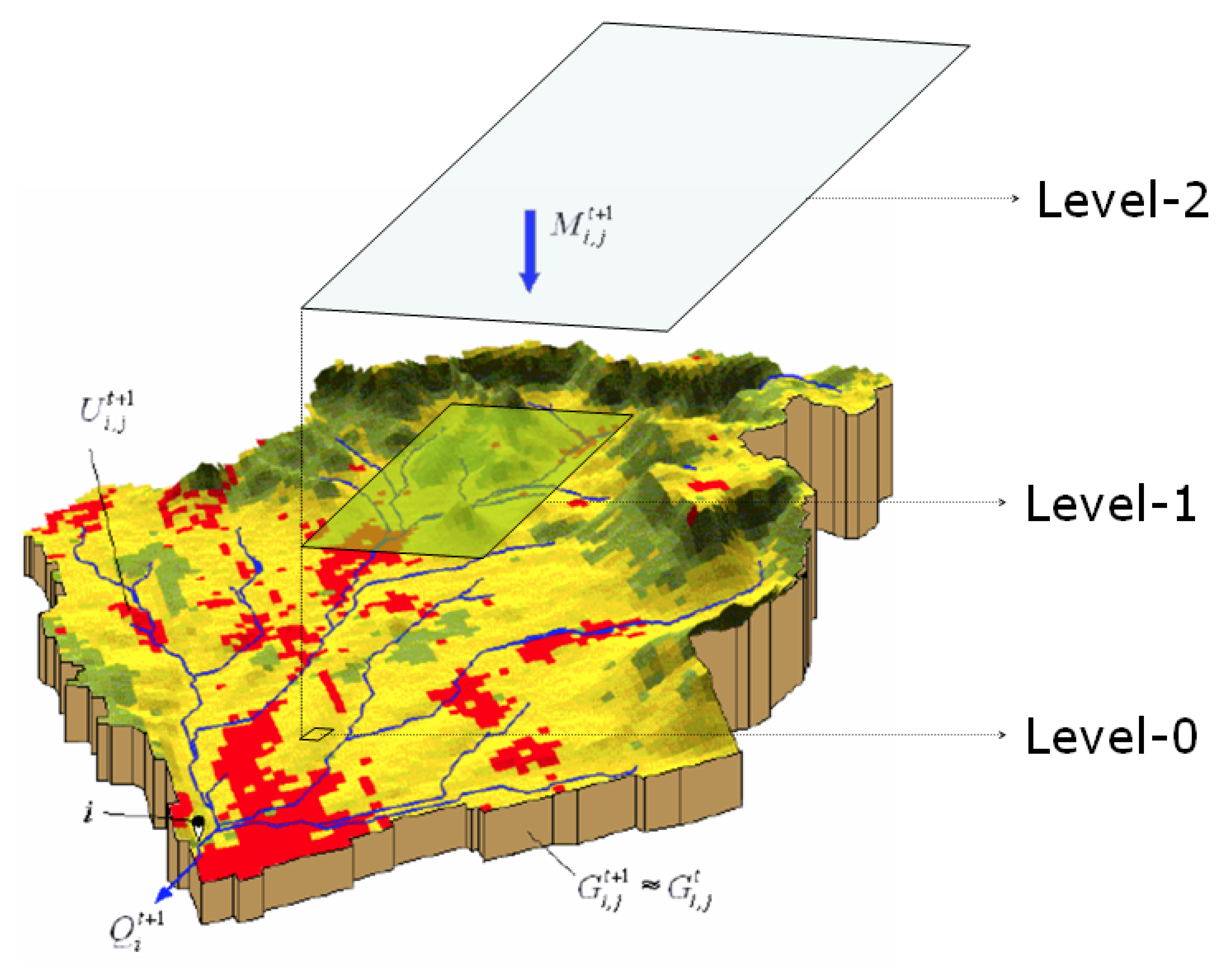
Dominant processes of the hydrological cycle at mesoscale span over several orders of magnitude [4] . In this model, three levels (mHM levels) will be differentiated to better represent the spatial variability of state and inputs variables:
A mesoscale basin is an open natural system, composed of very heterogeneous materials and having fuzzy boundary conditions. The continuity assumption of the the input variables is quite difficult to justify considering that the spatial heterogeneity of a basin is mostly described by discrete attributes such soil texture types, land cover classes, and geological formations. Due to these reasons, a system of ordinary differential equations ODEs was adopted to describe the evolution of the state variables at a given location \( i \) within the domain \( \Omega \). This system of ODE is
\begin{eqnarray*} \dot{x}_{1i} & = & P_i(t) - F_i(t) - E_{1i}(t) \\ \dot{x}_{2i} & = & S_i(t) - M_i(t) \\ \dot{x}_{3i}^l & = & (1-\rho^l) I_i^{l-1}(t) - E_{3i}^l(t) - I_i^l(t)\\ \dot{x}_{4i} & = & \rho^1 \big(R_i(t) + M_i(t)\big) - E_{2i}(t) - q_{1i}(t)\\ \dot{x}_{5i} & = & I_i^L(t) - q_{2i}(t)- q_{3i}(t)- C_i(t) \\ \dot{x}_{6i} & = & C_i(t) - q_{4i}(t) \\ \dot{x}_{7i} & = & \hat{Q}_{i}^{0}(t)-\hat{Q}_{i}^{1}(t) \end{eqnarray*}
\( \quad \forall i \in \Omega \).
where
| Variable | Description |
|---|---|
| Inputs | |
| \(P\) | Daily precipitation depth, \(\mathrm{mm}\; \mathrm{d}^{-1}\) |
| \(E_p\) | Daily potential evapotranspiration (PET), \(\mathrm{mm}\; \mathrm{d}^{-1}\) |
| \(T\) | Daily mean air temperature, \(^{\circ}C\) |
| Fluxes | |
| \(S\) | Snow precipitation depth, \(\mathrm{mm}\; \mathrm{d}^{-1}\) |
| \(R\) | Rain precipitation depth, \(\mathrm{mm}\; \mathrm{d}^{-1}\) |
| \(M\) | Melting snow depth, \(\mathrm{mm}\; \mathrm{d}^{-1}\) |
| \(E_p\) | Potential evapotranspiration, \(\mathrm{mm}\; \mathrm{d}^{-1}\) |
| \(F\) | Throughfall, \(\mathrm{mm}\; \mathrm{d}^{-1}\) |
| \(E_1\) | Actual evaporation intensity from the canopy, \(\mathrm{mm}\; \mathrm{d}^{-1}\) |
| \(E_2\) | Actual evapotranspiration intensity, \(\mathrm{mm}\; \mathrm{d}^{-1}\) |
| \(E_3\) | Actual evaporation from free-water bodies, \(\mathrm{mm}\; \mathrm{d}^{-1}\) |
| \(I\) | Recharge, infiltration intensity or effective precipitation, \(\mathrm{mm}\; \mathrm{d}^{-1}\) |
| \(C\) | Percolation, \(\mathrm{mm}\; \mathrm{d}^{-1}\) |
| \(q_{1}\) | Surface runoff from impervious areas, \(\mathrm{mm}\; \mathrm{d}^{-1}\) |
| \(q_{2}\) | Fast interflow, \(\mathrm{mm}\; \mathrm{d}^{-1}\) |
| \(q_{3}\) | Slow interflow, \(\mathrm{mm}\; \mathrm{d}^{-1}\) |
| \(q_{4}\) | Baseflow, \(\mathrm{mm}\; \mathrm{d}^{-1}\) |
| Outputs | |
| \(Q_{i}^{0}\) | Simulated discharge entering the river stretch at cell \(i\), \(\mathrm{m}^3\;\mathrm{s}^{-1}\) |
| \(Q_{i}^{1}\) | Simulated discharge leaving the river stretch at cell \(i\), \(\mathrm{m}^3\;\mathrm{s}^{-1}\) |
| States | |
| \(x_1\) | Depth of the canopy storage, \(\mathrm{mm}\) |
| \(x_2\) | Depth of the snowpack, \(\mathrm{mm}\) |
| \(x_3\) | Depth of soil moisture content in the root zone, \(\mathrm{mm}\) |
| \(x_4\) | Depth of impounded water in reservoirs, water bodies, or sealed areas, \(\mathrm{mm}\) |
| \(x_5\) | Depth of the water storage in the subsurface reservoir, \(\mathrm{mm}\) |
| \(x_6\) | Depth of the water storage in the groundwater reservoir, \(\mathrm{mm}\) |
| \(x_7\) | Depth of the water storage in the channel reservoir, \(\mathrm{mm}\) |
| Indices | |
| \(l\) | Index denoting a root zone horizon, \(l=1,\ldots,L\) (say \(L=3\)), in the first layer, \(0 \leq z \leq z_1\) |
| \(t\) | Time index for each \(\Delta t\) interval |
| \(\rho^l\) | Overall influx fraction accounting for the impervious cover within a cell |
mHM requires at most 28 parameters (depending of the configuration) per cell to account for the spatial variability of the dominant hydrological processes at a mesoscale river basin. These effective parameters have to be estimated through calibration. Calibrating this model with a significant number of free parameters for every grid cell would lead to over-parameterization in a mesoscale catchment. This, in turn, would tend to increase the predictive uncertainty of the model due to the equifinality [3] of feasible solutions. Moreover, the high dimensionality of this optimization problem is also a daunting task for the state-of-the-art optimization algorithms [14] . To overcome this problem a multiscale parameter regionalization (MPR) was employed in the mHM model [16] .
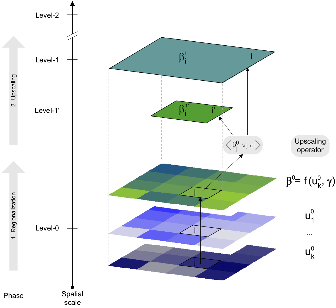
Based on this regionalization method, model parameters at a coarser grid (Level-1) are linked with their corresponding ones at a finer resolution (Level-0) (MPR). The linkage is done with upscaling operators. Model parameters at the finer scale are, in turn, regionalized with nonlinear transfer functions that couple catchment descriptors with the global parameters. Process understanding and empirical evidence are used to define these a priori relationships. The general form of an upscaling operator \(\mathrm{O}\) is:
\[ \beta_{ki}(t)= \mathrm{O}_k \Big \langle \beta_{kj}(t) \quad \forall j \in i \Big \rangle_{i} \]
where
\[ \beta_{kj}(t)= f_k \Big( u_j(t), \gamma \Big). \]
Here \(k=1,\ldots,K\) with \(K\) denoting the number of distributed model parameters. \( u_j\) denotes a \(v\)-dimensional predictor vector for cell \(j\) at level-0 which is contained by cell \(i\) at level-1 (e.g. land cover, elevation, soil texture).
\( \gamma \) is a \(s\)-dimensional vector of transfer parameters(super parameters), with \(s\) denoting the number of free parameters to be calibrated or total degrees of freedom. \(\mathrm{O}_k \langle \bullet \rangle_{i}\) denotes the kind of operator applied for the regionalization of the parameter \(k\). Several types of operators were employed, e.g. majority \(\mathcal{M}\), arithmetic mean \(\mathcal{A}\), maximum difference \(\mathcal{D}\), geometric mean \(\mathcal{G}\), and harmonic mean \(\mathcal{H}\). This table also shows the type of relationship employed for the transfer function and the predictors. By establishing such a relationships, the calibration algorithm finds good solutions for the transfer functions parameters ( \(s=\) 45) instead of the model parameters for every grid cell. This, in turn, implies a great reduction of complexity since \( K \times n \gg s\), where \(n\) denotes the total number of cells of a given basin at level-1.
Let \(\mathbf{M}\{\mathbf{f},\mathbf{g}\}\) be a dynamic, spatially distributed, parameter efficient, integrated model that relates a number of state variables \(\mathbf{x}\) with some observables called: inputs \(\mathbf{u}\) and outputs \(\mathbf{y}\). In general, the system is described by the following system of equations
\begin{eqnarray*} \dot{\mathbf{x}}(i,t) & = &\mathbf{f}(\mathbf{x},\mathbf{u}, \beta, \gamma )(i,t) + \eta(i,t)\\ \mathbf{y}(i,t) &=& \mathbf{g}(\mathbf{x}, \mathbf{u}, \beta, \gamma )_{\Omega} + \epsilon(i,t)\\ \end{eqnarray*}
where
In general, \(\gamma\) can be estimated, for example, by
\[ \min_{\hat{{\gamma}}}=\|\mathbf{y} -\mathbf{\hat{y}}\| \]
where \(\|\cdot\|\) denotes a robust estimator. Many procedures to estimate global parameters are provided in mHM (e.g. simulated annealing [1], dynamically dimensioned search [17] . Other techniques can be found in the CHS Fortran Library.
Good parameter sets for \( \gamma \) were identified with a split-sampling technique using an adaptive constrained optimization algorithm based on simulated annealing (SA) [1] . The overall model efficiency was estimated as a weighted combination of four estimators based on the Nash-Sutcliffe efficiency (NSE) between observed and calculated streamflows using three different time scales (daily, monthly and annual) as well as the logarithms of the streamflow to downplay the effects of the peak flows over the low flows [10] . These objective functions are denoted by \(\phi_k,\, k=1,4\). Every objective function should be normalized in the interval [0,1], with 1 representing the best posible solution. The overall objective function to be minimized is then
\[ \Phi = \Big(\sum_i w_i^p (1-\phi_i)^p \Big)^{\frac{1}{p}} \]
where \(p>1\), and \(\sum_{i=1}^4 w_i =1\). Here \(p\) is an exponent according to the compromise programming technique [9] and \(w_i\) denote the degree of importance of each objective. High values of \(p\), say \(p=6\), should be chosen to avoid substitution of objective function values at low levels. In general, the estimators related to daily streamflows were twice as important as the long-term ones, thus \(\{w_i\}=\{\frac{2}{4},\frac{1}{4},\frac{1}{4},\frac{2}{4} \}\). The NSE for a given time interval \(t'\) is given by
\[ \phi_k = 1 - \frac{\displaystyle \sum_{t'} \left(y_k(t') - \hat{y}_k(t')\right)^2} {\displaystyle \sum_{t'} \left(y_k(t') - \overline{y}_k(t')\right)^2 } \]
where \(\overline{y}_k(t')\) is the mean value of the observations time series over the calibration period. The index \(k\) denotes here the daily, monthly, yearly, and the transformed \(\ln y(t)\) streamflow discharges. \(y\) and \(\hat{y}\) denote the observed and simulated streamflows at a given time scale. Fruther details about mHM's calibration options can be found in the section Calibration Options.
Data Preparation for mHM (see Data Preparation for mHM)
mHM comes with a test basin. For details see The details about the test basin.
To set up a new input data for mHM see Protocols for setting up a new mHM basin.