5.13.2-dev0
|
mHM
The mesoscale Hydrological Model
|
|
mHM
The mesoscale Hydrological Model
|
To run mHM the user requires a number of datasets. The follwing subsection gives a short overview and references to freely available datasets.
Meteorological data is usually available from the weather services of the countries of modelling interest. Freely available alternatives are the EOBS (http://www.ecad.eu/download/ensembles/download.php) and the WATCH datasets (http://www.eu-watch.org/gfx_content/documents/README-WFDEI.pdf).
You may have difficulties finding measurement data for Potential Evapotranspiration (PET). One possible solution, would be to calculate PET from the much easier available variables mean, maximum and minimum air temperature, using the Hargreaves-Samani method.
The two meteorological variables which are needed:
| Name | Unit | Temporal resolution |
|---|---|---|
| Precipitation | \(\mathrm{mm}\) | hourly to daily |
| Average air temperature | \(^\circ \mathrm{C}\) | hourly to daily |
Dependent of the specification for the potential evapotranspiration (processCase(5)) additional meteorological variables may be need:
| Name | Unit | Temporal resolution |
|---|---|---|
| 0 - Potential evapotranspiration | \(\mathrm{mm}\) | hourly to daily |
| 1 - Minimum air temperature | \(^\circ \mathrm{C}\) | daily |
| 1 - Maximum air temperature | \(^\circ \mathrm{C}\) | daily |
| 2 - Net radiation | \( W\;m^{-2} \) | daily |
| 3 - Net radiation | \( W\;m^{-2} \) | daily |
| 3 - Absolut vapur pressure of air | \( Pa \) | daily |
| 3 - Windspeed | \( m\;s^{-1} \) | daily |
In addition to the Digital Elevation Models (DEM) usually provided by federal authorities, a number of free alternatives exists. SRTM data is available from 60° South to 60° North in a 3" (~ 90 m) resolution (http://srtm.csi.cgiar.org/), the ASTER-GDEM covers the entire globe with a resolution of 1" (http://gdem.ersdac.jspacesystems.or.jp/). Hydrographically corrected SRTM data and a number of derived products in different resolutions are available from the HydroSHEDS project (http://hydrosheds.cr.usgs.gov/index.php).
Soil and hydrogeological data is usually provided by the geological surveys. On the soil side the Harmonized World Soil Database would be a free alternative (http://webarchive.iiasa.ac.at/Research/LUC/External-World-soil-database/HTML/).
| Name | Unit | Temporal resolution |
|---|---|---|
| Digital elevation model | \(\mathrm{m}\) | - |
| Soil maps with textural properties (% sand and clay contents, bulk density per horizon, and root depth zone) | - | - |
| Geological maps with aquifer properties (specific yield, permeability, aquifer thickness) | - | - |
| Streamflow location | \((\mathrm{m}, \mathrm{m})\) (lat,lon) | - |
Free land cover data is available from different sources. The Corine programm provides land cover scenes for Europe with resolutions of 100m and 250m (http://www.eea.europa.eu/publications/COR0-landcover), the Global Land Cover Map 2000 a dateset covers the entire world in a resolution of 1km.
| Name | Unit | Temporal resolution |
|---|---|---|
| Land cover scenes | - | monthly to annual |
| Leaf area index | - | weekly to monthly |
Streamflow measurments should also be available from federal authorities. In addition, the Global Runoff Data Center provides timeseries of varying length for several thousand gauging stations all over the world (http://www.bafg.de/GRDC)
| Name | Unit | Temporal resolution |
|---|---|---|
| Streamflow measurements | \(\mathrm{m}^3 \mathrm{s}^{-1}\) | hourly to daily |
| Name | Unit | Temporal resolution |
|---|---|---|
| Snow cover | - | daily to weekly |
| Land surface temperature | \(\mathrm{K}\) | daily to weekly |
| Groundwater station location | \((\mathrm{m}, \mathrm{m})\) (lat,lon) | - |
| Groundwater head measurements | \(\mathrm{m}\) | weekly to monthly |
| Eddy covariance station location | \((\mathrm{m}, \mathrm{m})\) (lat,lon) | - |
| Eddy covariance measurements | \(\mathrm{m}\) | hourly |
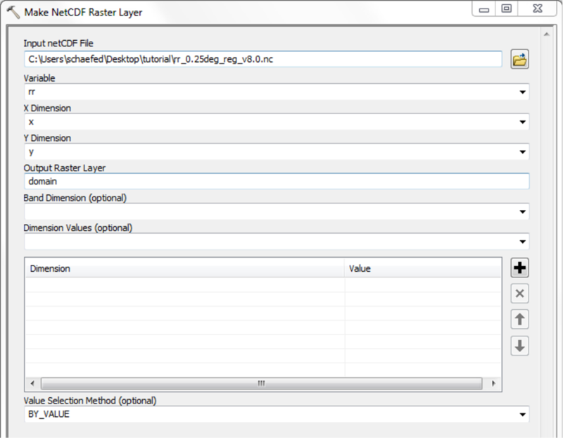
Forcing data should be available from federal databases like DWD for Germany. Be sure to bring data in the netcdf format, like
These files can be edited with the CDO module package in order to select or change data. Please read the according CDO and NCKS reference sheets for details and make sure to load the CDO modules before starting.
Let FULLMAP.nc be the the forcing data of a region much greater than your catchment. Let X1, X2, Y1, Y2 be the coordinates (lon and lat) of a rectangular overlapping the catchment. The forcing data MAP.nc for your catchment can be extracted by the CDO command:
Optionally, certain pixels can be extracted, too:
Let MAP.nc be the forcing data including your period of interest. Let DATE1 and DATE2 be the starting and ending dates of your period, respectively. Their date format is YYYY-MM-DD. The data PERIOD.nc can be extracted by the CDO command:
Please note that a reference date according to DATE1 should be provided in PERIOD.nc:
Any data provided for mHM should be of the data type DOUBLE. You should convert all data related to a variable VAR (e.g. tavg) with the following CDO command:
The only exception here is the time, its data type has to be INTEGER. This can be changed with NCAP2:
In mHM the variable names of the forcing are hard-coded. They need to be
For example, you can change the variable name TEMPERATURE in your NETCDF file with the following CDO command:
Every meteorological data file should come with an additional file "header.txt" in the same directory. In the following example, we has only one pixel of data (ncols=nrows=1) and a cell size of 4km. The easting and northing coordinates of the lower left cornaer should be similar to the morphological data of your catchment.
In order to be consistent in your data, you should specify the same NODATA value everywhere. For example, specify "-9999" in your header file as NODATA value. Usually, this should be changed also in NC files by the ncatted command. The following example overwrites or adds (o) the NODATA attribute "_FillValue" with value "-9999" of type double (d) to the variable "pre":
As input mHM additionally needs a latlon.nc file specifying the geographical location of every grid cell in WGS84 coordinates. This file has to be adjusted for every resolution of the level-1 hydrological simulations.
For creating a latlon file mHM comes with the python script create_latlon.py, which can be found in pre-proc/. Detailed information for the usage of this python script can be found in the online help by typing:
create_latlon.py needs several specifications via command line switches. First, the coordinate system of the morphological and meteorological data have to be specified according to www.spatialreference.org by using the switch: -c. Second, you need to specify three header files containing the corresponding information for the different spatail resolutions connected to mHM. The three resolutions are the resoltution of 1) the morphological input (switch: -f), 2) the hydrological simulation (switch: -g), and 3) the routing (switch: -e).
These header files can be produced by adopting the header file of the meteorological data Therefore, copy one of these files that you generated for meteo data (see Preparation of the Forcings):
Edit the new file header.txt such that cellsize equals your hydrologic resolution. You have to adapt ncols and nrows to that resolution such that it covers the whole region. For example, reducing the cell size from 2000 to 100, the number of columns and rows should be increased by a factor of 20.
Third, you need to set the path and filename for the resulting output file by using the switch -o.
An example for creating a lat-lon-file looks like
Keep in mind that you need one latlon file for each hydrologic resolution in mHM. Since the filename latlon.nc is hard-coded in mHM, we recommend to create different directories for each resolution you need, containing the related header and latlon file.
MHM needs several morphological input datasets. All these have to be provided as raster maps in the ArcGis ascii-format, which stores the above header and the actual data as plain text. Some of the raster files need to be complemented by look-up tables providing additional information. The tables and their structure are described in more detail in subsection Table Data. Take care of the follwing limitations to mHM input data during data processing:
The required datasets and their corresponding filenames:
| Description | Raster file name | Table file name |
|---|---|---|
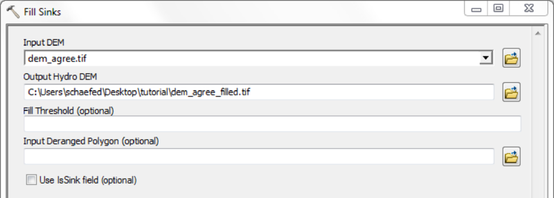
| Sink filled Digital Elevevation Model (DEM) | dem.asc | - |
| Slope map | slope.asc | - |
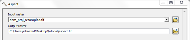
| Aspect Map | aspect.asc | - |
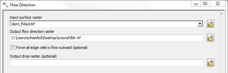
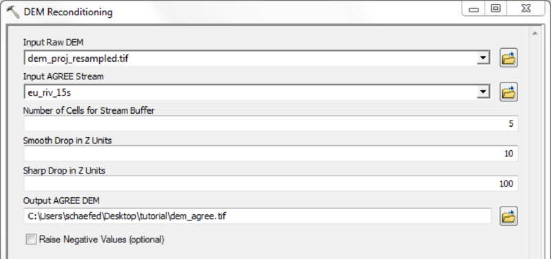
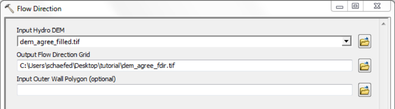
| Flow Direction map | fdir.asc | - |
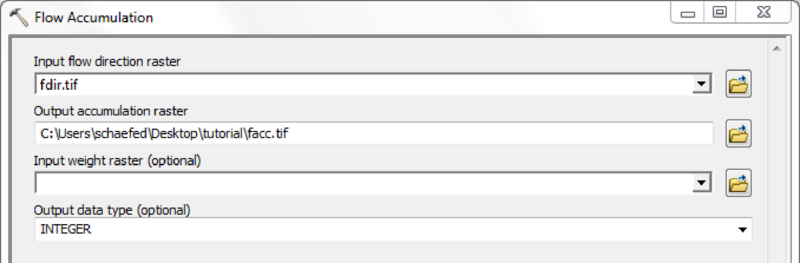
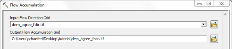
| Flow Accumulation map | facc.asc | - |
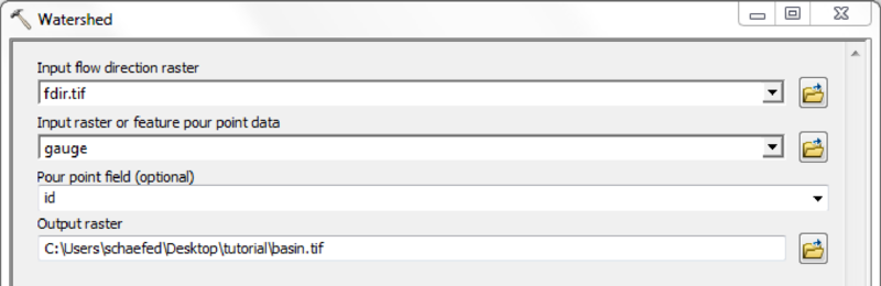
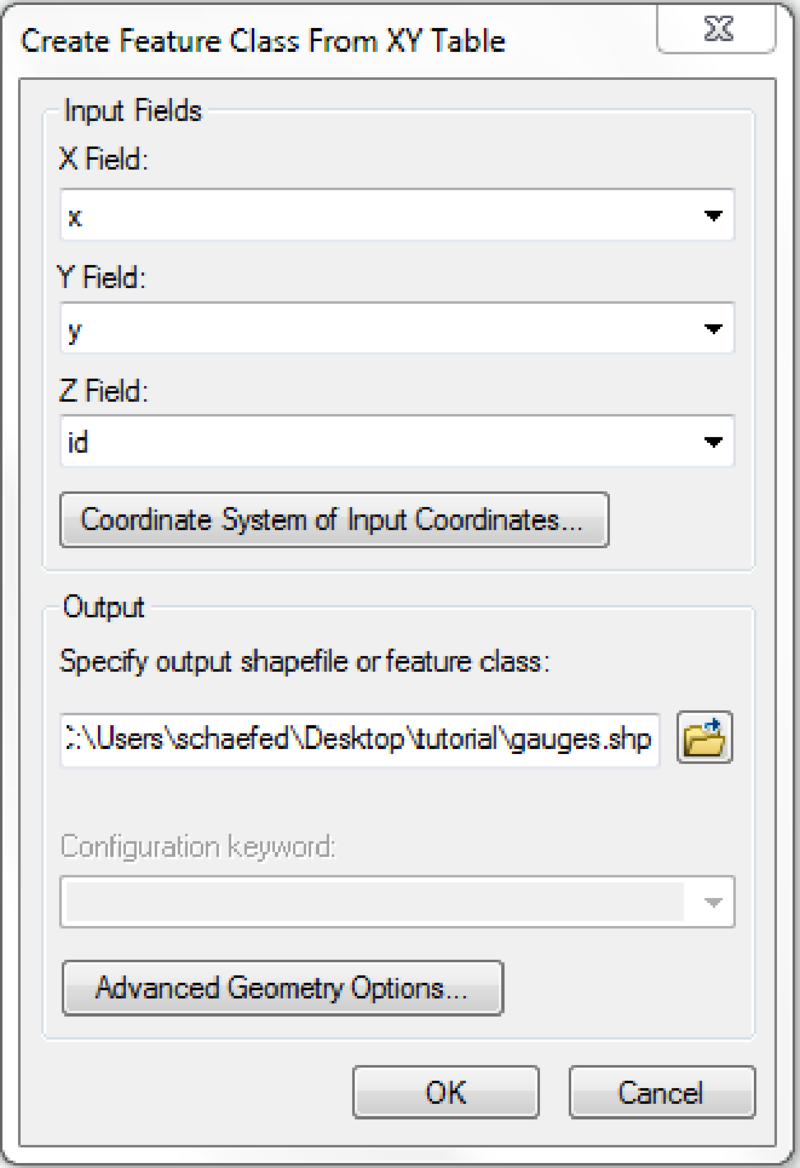
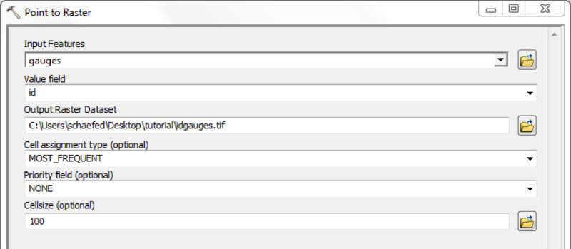
| Gauge(s) position map | idgauges.asc | [gauge-id].txt |
| Soil map | soil_class.asc | soil_classdefinition.txt |
| Hydrogeological map | geology_class.asc | geology_classdefinition.txt |
| Leaf Area Index (LAI) map | LAI_class.asc | LAI_classdefinition.txt |
| Land use map | your choice | - |
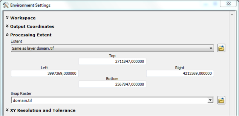
In the following paragraphs a possible GIS workflow is outlined using the software ArcMAP 10 with the Spatial Analyst Extension and optionally the Arc Hydro Tools (http://downloads.esri.com/blogs/hydro/AH2/ArcHydroTools_2_0.zip)
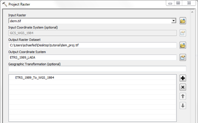
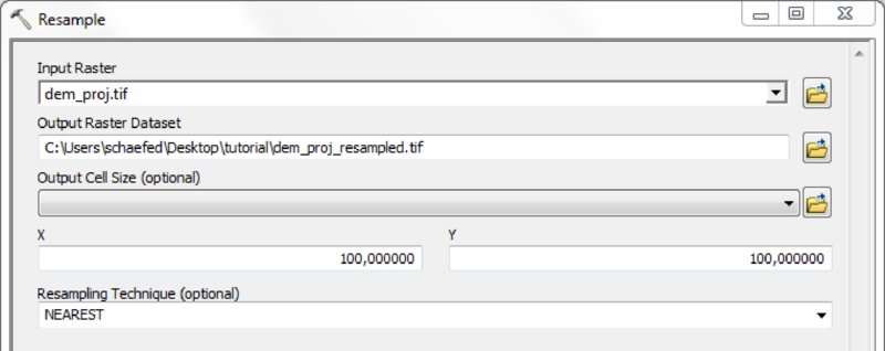
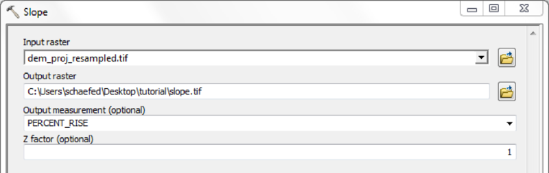
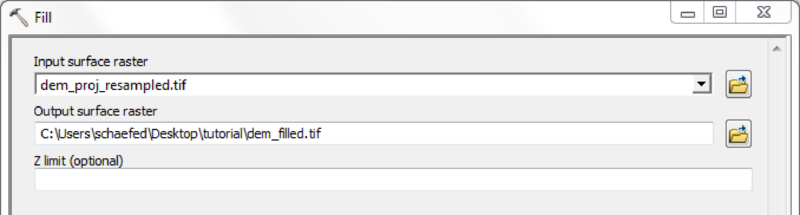
Depending on quality and resolution of the DEM map, these steps can be done with the respective tools from the Spatial Anaylst Extension or by using the Arc Hydro Tools.
If a high quality DEM, with a resolution fine enough to represent small scale river morphology is available, you may calculate flow direction and flow accumulation directly.
Using the Arc Hydro Tools is recommended in case of doubtful DEM quality and/or coarse map resolutions.
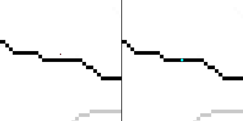
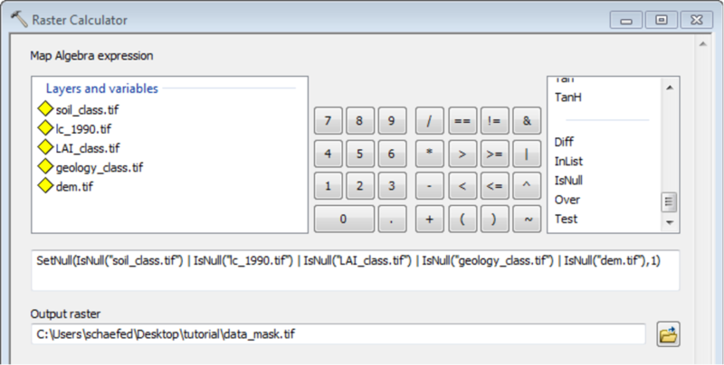
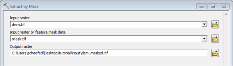
Mask all mHM input raster files with the created watershed mask
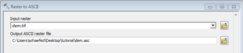
Convert the processed and masked raster maps into ASCII files
Unlike the other classified datasets (soils, hydrogeology, LAI), where as much information as available can be added, the land use data is restricted to three different classes, which are listed below:
| Class | Description |
|---|---|
| 1 | Forest |
| 2 | Impervious |
| 3 | Pervious |
As previously stated, the input datasets 'soil_class.asc', 'geology_class.asc', 'idgauges.asc' and 'LAI_class.asc' need to be complemented by look-up-tables. All these look-up tables specify the total number of classes/units to read in the very first line, following the keywords 'nSoil_Types', 'nGeo_Formations' and 'NoLAIclasses' respectively. The second line acts as a header describing the contents of the following data. In the subsection The soil look-up table The hydrogeolgy look-up table and The LAI look-up table screenshots of shorted, but sufficient table files are presented. All fields are further listed and described in the repective tables.
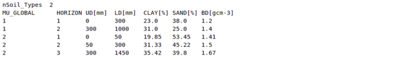
| Field | Description |
|---|---|
| MU_GLOBAL | Soil id as given in the corresponding 'soil_class.asc' map. All raster map ids must be given here |
| HORIZON | Horizon number starting at the top of the soil column. Your are free to provide any number of horizons for each soil individually |
| UD[mm] | Upper depth of the horizon in millimeter. Should be 0 for the first, and the lower depth of the superimposing horizon for all others |
| LD[mm] | Lower depth of the horizon in millimeter |
| CLAY[%] | Clay content in percent |
| SAND[%] | Sand content in percent |
| BD[gcm-3] | Mineral bulk density in grams per cubic centimeter |

| Field | Description |
|---|---|
| GeoParam(i) | Parameter number of the formation, the link to 'mhm_parameter.nml' |
| ClassUnit | Class id as present in the 'hydrogeology_class.asc' raster map |
| Karstic | Presence of karstic formation (0: False, 1: True) |
| Description | Text description of the unit |
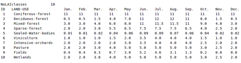
| Field | Description |
|---|---|
| ID | LAI class id as given in the file LAI_class.asc |
| LAND-USE | Description of the LAI class |
| Jan. to Dec. | Monthly LAI values |
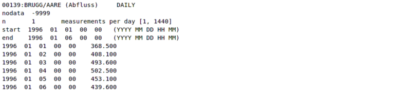
The structure of the gauge files is different from the look-up tables listed so far. The following table describes its content.
| Line | Description |
|---|---|
| 1 | Gives basic information about the gauging station (Station-Id:Station-Name/River-Name) |
| 2 | Specifies the nodata value |
| 3 | The number of measurements per day |
| 4 | The start date of the time series in the format given in parentheses |
| 5 | The end date of the time series in the format given in parentheses |
| 6 to end | The measurement data in cubic meter per second preceded by the actual date in the same format as the dates of lines four and five |
For every gauge id given in 'idgauges.asc' one gauge file has to be created as outlined above. The file name has to exactly reflect the gauge id and carry a '.txt' extension. The table data file for a gauge with an id of 0343 in 'idgauges.asc' should therfore be named '0343.txt'.
Make sure that all decimals are indicated with dots, not commas:
Make sure that accuracy of your llcorners is reasonable. For example, the following code removes all but one digits after the dot:
Make sure that your files cover the same spatial domain. In case your grid origins match, but you are missing rows and columns, the perl script pre-proc/enlargegrid.pl will pad your data at the top and the right end of the grid.
If your data differs more substantially the program 'mHM/pre-proc/resize_grid.py' will harmonize your grids.
The script takes three Input arguments:
The program will fail, if your target grid is smaller than the source grid or if the cellsizes of both grids are not divisable. If necessary the source grid will be shifted in order to make both origins match. This 'shift' is only accomplished by changing the values of the corner coordinates, no real interpolation will be done.